AxoBench metrics
Error anatomy
Break a prediction's errors down by spike outcome, time from a spike, firing rate, frequency band, and morphology.
The core metrics state how large an error is; the error anatomy shows where it comes from. error_anatomy uses the scored traces of the evaluator, with the same calibrated spike threshold, predicted spike events, action-potential windows, and relevance, so every part adds up to the metrics in the report. It requires AxoBench 0.2.1.
Example: AxoSim–GRU Medium
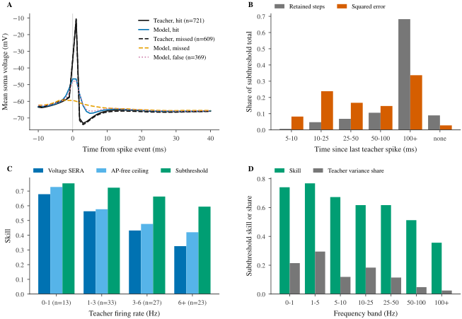
Error anatomy of AxoSim–GRU Medium on the confirmation block of val: validation_sample_start=120, 120 traces balanced over the five morphologies, of which 24 calibrate the spike threshold (calibration_fraction=0.2) and 96 are scored after the first 500 steps. Written by axobench error-anatomy from the model's evaluation cache. Select the figure to open it at full size.
The sections below read this example. All values are taken from the command’s error-anatomy.json.
Spike events
Teacher spikes and predicted spike events are matched one to one, as for spike F1. Within HIT_TOLERANCE_STEPS (2 ms), a matched teacher spike is a hit, an unmatched teacher spike is a miss, and an unmatched predicted spike is a false spike. The section also lists F1 per tolerance and the timing errors, predicted minus teacher step, of the events matched within the widest tolerance.
| Quantity | Value |
|---|---|
| Teacher spikes | 1,962 |
| Predicted spikes | 1,669 |
| Hits, misses, false spikes (2 ms) | 1,110, 852, 559 |
| F1 at 0 ms and 5 ms | 0.227, 0.725 |
| Matched within 5 ms; offset 0, −1, +1 ms | 1,316; 408, 255, 251 |
The model predicts 15% fewer spikes than the teacher, and misses outnumber false spikes. The timing errors are symmetric around zero, so the low exact-time F1 reflects jitter of about 1 ms rather than a systematic lag; a constant lag would shift the distribution to one side.
Spike-triggered voltage
Panel A averages the unclipped teacher voltage and the model voltage around isolated events: no other event of the same train lies within STA_LAGS_STEPS, 10 steps before to 40 after. Averaging around hits, misses, and false spikes separates three questions: does the model emit an action potential where it predicts a spike, what does it do where it misses one, and what does a false spike look like.
| Events | Count | Teacher peak | Model peak |
|---|---|---|---|
| Hit | 721 | −10.6 mV | −46.6 mV |
| Missed | 609 | −11.0 mV | −59.2 mV |
| False | 369 | −55.0 mV | −47.6 mV |
At hits the spike channel is right, but the voltage channel peaks at −46.6 mV where the teacher reaches −10.6 mV: the model marks the spike without the action-potential waveform. A model that averages action potentials away in this way loses most of the Voltage SERA, which is dominated by action-potential windows, and stays near the AP-free ceiling. After hits the teacher falls to −73.1 mV 3 ms after the spike, the model only to −67.2 mV 5 ms after it, so the afterhyperpolarization is too shallow. At misses the model voltage stays near −59.5 mV through the teacher spike, with neither a peak nor an afterhyperpolarization. Around false spikes the teacher’s mean voltage stays between −64 and −55 mV; its maximum of −55.0 mV lies 4 ms after the event, which suggests that some false spikes are teacher spikes predicted more than 2 ms too early rather than spikes in quiet periods. The timing errors above count these within 5 ms.
Subthreshold error by spike distance
The subthreshold RMSE is broken down by time since the last teacher spike and, separately, until the next one, in bins of 0–5, 5–10, 10–25, 25–50, 50–100, and 100+ ms, and none for steps without such a spike. Each bin reports its share of retained steps, its share of squared error, its share of the null prediction’s squared error, and its skill. The 0–5 ms bin after a spike is empty because the action-potential window excludes those steps.
| Since last teacher spike | Retained steps | Squared error | Skill |
|---|---|---|---|
| 5–10 ms | 0.6% | 8.2% | 0.13 |
| 10–25 ms | 4.8% | 23.8% | 0.39 |
| 25–50 ms | 6.8% | 16.7% | 0.51 |
| 50–100 ms | 10.6% | 14.7% | 0.62 |
| 100+ ms | 68.3% | 33.7% | 0.77 |
| none | 9.0% | 2.8% | 0.79 |
The 5.4% of retained steps within 25 ms after a spike carry 32% of the squared error. Error concentrated shortly after spikes points to the spike: a too-shallow afterhyperpolarization, as panel A shows, or a missed spike, whose waveform and recovery the model does not produce. Error spread evenly over time would instead point to offset or gain errors. Measured until the next spike, the error is not concentrated: 0.6% of the steps lie within 5 ms before a spike and carry 2.4% of the error, with skill 0.70, so the depolarization before a spike is reproduced about as well as the rest of the trace.
Skill by firing rate and morphology
Traces are grouped by their teacher firing rate, 0–1, 1–3, 3–6, and 6+ Hz, and by morphology. Each group reports Voltage SERA skill, the AP-free ceiling, skill as a fraction of the ceiling, Dynamics SERA skill, subthreshold skill, and Mean F1, with relevance and references fixed by the whole block. Dataset-relative skill defines these quantities.
| Teacher rate | Traces | Voltage SERA skill | Ceiling | Skill / ceiling | Subthreshold skill | Mean F1 |
|---|---|---|---|---|---|---|
| 0–1 Hz | 13 | 0.68 | 0.73 | 0.93 | 0.75 | 0.59 |
| 1–3 Hz | 33 | 0.56 | 0.58 | 0.98 | 0.72 | 0.63 |
| 3–6 Hz | 27 | 0.43 | 0.48 | 0.91 | 0.66 | 0.60 |
| 6+ Hz | 23 | 0.33 | 0.42 | 0.77 | 0.59 | 0.53 |
The ceiling falls with the rate because more of the trace lies in action-potential windows, so raw skill falls even for a model that is equally good relative to what is achievable without action potentials. The fraction of the ceiling separates the two effects: here it drops only in the 6+ Hz bin, together with subthreshold skill and Mean F1, so the model also degrades at high rates beyond the ceiling effect. By morphology the fraction ranges from 0.75 for specimen_479770916, whose traces fire at 7.5 Hz on average, to 1.02 for specimen_488683425 at 2.2 Hz. A fraction above 1 is possible because a model that does emit action potentials can exceed the AP-free ceiling.
Subthreshold skill by frequency band
The retained subthreshold error and the teacher’s deviation from its per-trace mean are zero-filled outside the retained steps and split into frequency bands by Parseval’s theorem: 0–1, 1–5, 5–10, 10–25, 25–50, 50–100, and 100+ Hz. Each band reports its share of the error power, its share of the teacher’s variance, and its skill.
In the example, skill is 0.74 and 0.77 in the two lowest bands, which hold 51% of the teacher variance, and falls to 0.62 at 10–50 Hz, 0.51 at 50–100 Hz, and 0.36 above 100 Hz. The 10–25 Hz band holds 24.9% of the error power but 18.4% of the teacher variance. Slow drifts are reproduced; the fast fluctuations of synaptic input are smoothed. Zero-filling the excluded windows leaks some power between bands, so compare bands within one evaluation rather than reading absolute spectra.
Run from the command line
axobench error-anatomy reads an evaluation cache and the targets of the cached block:
axobench error-anatomy \
  --cache runs/gru-medium/axobench-evaluation-cache.npz \
  --targets runs/confirmation-block-targets.npz \
  --output runs/gru-medium/anatomy \
  --formats svg,png
The cache is the file written by write_model_evaluation_cache or axosim-evaluate-model --save-cache, or any NPZ with a prediction array. The targets file holds target and optionally raw_soma_mv and trace_ids, in the cache’s trace order; without --targets they are read from the cache file. The command fails unless the targets match the target hash and trace IDs recorded in the cache. ignore_start and the calibration fraction come from the cache’s protocol, so the anatomy uses the evaluator’s split; --ignore-start and --calibration-fraction override them. Save the targets of a block you scored yourself with np.savez(path, target=target, raw_soma_mv=raw_soma_mv, trace_ids=np.array(trace_ids)).
The command writes:
error-anatomy.json, the complete result;error-anatomy.<format>for each of--formats, by default PDF and PNG;error-anatomy.tex, a standalone pgfplots version of the same four panels.
It prints the output paths with the overall Voltage SERA skill, ceiling, skill of ceiling, subthreshold skill, and Mean F1.
Use it from Python
error_anatomy takes the arrays and settings of evaluate_predictions:
import numpy as np
from axobench.benchmark import EvaluationConfig, error_anatomy
from axobench.benchmark.plots import plot_error_anatomy

with np.load("runs/gru-medium/axobench-evaluation-cache.npz") as cache:
    prediction = cache["prediction"]
with np.load("runs/confirmation-block-targets.npz") as block:
    target, raw_soma_mv = block["target"], block["raw_soma_mv"]
    trace_ids = [str(i) for i in block["trace_ids"]]

anatomy = error_anatomy(
    prediction, target, raw_soma_mv=raw_soma_mv, trace_ids=trace_ids,
    config=EvaluationConfig(calibration_fraction=0.2),
)
events = anatomy["spike_events"]
print(events["hit"], events["missed"], events["false"])
print(round(anatomy["overall"]["voltage_sera_skill"], 3))
plot_error_anatomy(anatomy, "runs/gru-medium/anatomy/error-anatomy", formats=("pdf",))
1110 852 559
0.423Pass the EvaluationConfig of the evaluation you want to explain; the GRU Medium cache was written with a calibration fraction of 0.2 rather than the default 0.25. The result is JSON-serializable, with times in steps or milliseconds and voltages in millivolts; the error anatomy reference lists every field.
Export for LaTeX
plot_error_anatomy writes the figure with Matplotlib in the AxoBench paper style, STIX serif text and the Okabe–Ito palette, and, unless tikz=False, a standalone pgfplots document of the same panels and data. The .tex file compiles on its own, for example with tectonic error-anatomy.tex, and its groupplot can be copied into a paper so the figure uses the document’s fonts. Colors are defined as abblue, aborange, and so on from the same palette.
Next steps
Compare models on a common rate distribution with dataset-relative skill, or return to the diagnostics for the attention panel and diagnostic rows.